
The Tropical Cyclone Formation Probability (TCFP) product amalgamates multiple data sources to generate short-term forecasts of global tropical cyclogenesis. The forecasts are a probability of tropical cyclone formation within 500 km of each grid point for the domain extending from 45° S to 45 °N and 0°E to 360 °E. The fourth version of the algorithm uses water vapor imagery with a central wavelength near 6.7 µm from the global constellation of geostationary satellites [e.g., the GOES-R series (GOES-16/-17/-18), Himawari-8/-9, Meteosat Second Generation (Meteosat-8/-9/-10/-11), and Meteosat Third Generation], sea surface temperature observations from the Group for High Resolution Sea Surface Temperature (GHRSST) Level 4 analysis, and forecast fields of wind, temperature, and moisture from the NOAA/NCEP Global Forecast System. The product domain is divided into 7 main basins (below) based on satellite coverage and warning agency boundaries.
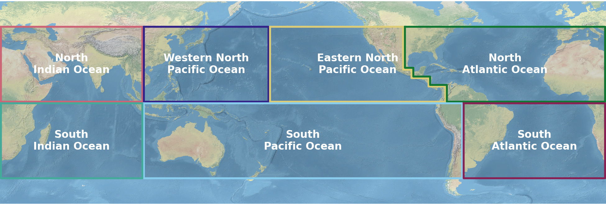
Figure: The Tropical Cyclone Formation Probability product domain and basins.
Input parameters:
Geostationary Satellite:
- PCCD: The percent of channel water vapor pixels less than -40 °C within 500 km of a grid point.
- BTWM: The average water vapor brightness temperature greater than -40 °C within 500 km of a grid point.
- Ocean:
- RSST: The average sea surface temperature within 50 km of a grid point.
Large-scale Environmental:
- MSLP: The 200 to 800 km azimuthally averaged mean sea level pressure.
- HDIV: The 0 to 1000 km azimuthally averaged 850 hPa horizontal divergence.
- RVOR: The 0 to 1000 km azimuthally averaged 850 hPa relative vorticity.
- VSHS^: The 0 to 500 km azimuthally averaged 850-500 hPa shallow-layer vertical wind shear.
- VSHG: The 0 to 500 km azimuthally averaged 850-200 hPa generalized vertical wind shear.
- MWND^: The 850 to 200 hPa column-averaged mean wind within 500 km.
- TANM^: The 400 to 300 hPa temperature anomaly calculated using the 0 to 100 km and 1500 km temperature profiles.
- TADV: The 0 to 500 km azimuthally averaged 850 to 700 hPa horizontal temperature advection calculated from the geostrophic thermal wind equation.
- TGRD^: The 0 to 500 km azimuthally averaged 850 to 700 hPa horizontal temperature advection calculated from the geostrophic thermal wind equation.
- THDV*: The 200 to 800 km azimuthally averaged vertical instability parameter, defined as the vertical average temperature difference between the equivalent potential temperature of a parcel lifted from the surface to the equilibrium level, and the saturation equivalent potential temperature of the environment.
- CIN^: Convective inhibition calculated from 200 to 800 km.
- VVAC^: The average vertical velocity of an air parcel from rising from the surface to the level of neutral buoyancy calculated from an entrained plume cloud model using the 200 to 800 km temperature and relative humidity profiles.
^Predictor but not plotted
*Plotted variable but not predictor
Climatology:
Climatological input parameters are computed over the following time periods: Ocean: 1999 to 2023 using the Optimum Interpolation Sea Surface Temperature (i.e., Reynolds SST) through 2015 and the GHRSST product from 2016 through 2023. Geostationary satellite: 1999 to 2023 calculated from NOAA/NCEI Climate Data Record GridSat-B1 product. Note that near global coverage began around 1999. Large-scale Environmental: 1999 to 2023 from the Global Forecast System Final Analysis / Global Data Assimilation System
Algorithm methodology:
The formation probability algorithm is a multistep process. First, the algorithm interpolates the satellite, ocean, and model data onto cylindrical grids at each grid point and calculates the azimuthally averaged quantities before computing the derived metrics (e.g., vertical wind shear). Next, the algorithm screens points based on predetermined thresholds to avoid erroneous probabilistic output indicating genesis (e.g., over cool SSTs). Then, the algorithm makes a probabilistic prediction of genesis using an equally-weighted consensus of machine learning algorithms. TCFP uses random forest, linear regression, and linear discriminant analysis algorithms trained with global data and a linear regression and a linear discriminant analysis trained on individual ocean basins. Lastly, the algorithm generates output files for the probabilities and graphical output of both the probabilities and predictors.
Subregion information:
To provide some time continuity of the product, TCFP also includes plots showing the formation probability and the primary predictors over sub-basins for the Atlantic Ocean, Eastern and Western Pacific Ocean, and Indian Ocean basins. The time series products include a comparison of the current condition and climatology over the sub-basins.
Atlantic Ocean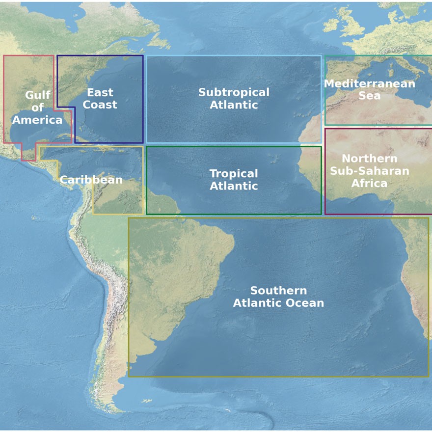 |
Eastern Pacific Ocean |
Western Pacific Ocean |
Indian Ocean |
| Figure: TCFP sub-basins | |||
Figure: The Tropical Cyclone Formation Probability product subbasins.
Reference: TCFP Algorithm Theoretical Basis Document